How To Change The Color Of Worksheet Gridlines In Excel

Struggling to manage your data in Excel? You’re not alone. Learn how to make it easier by customizing the color of gridlines, and make your spreadsheet look professional.

Accessing Excel Options to Change Worksheet Gridline Color

I’m an Excel fan, and I’m always seeking ways to make it better! Let’s look at how to switch the color of gridlines in Excel – a simple, yet successful manner to customize and boost the appearance of your spreadsheets. We’ll begin by launching Excel and finding the file tab. After that, we’ll learn to pick choices to alter the gridline color. With these steps, you can design great-looking and organized spreadsheets that will astound!

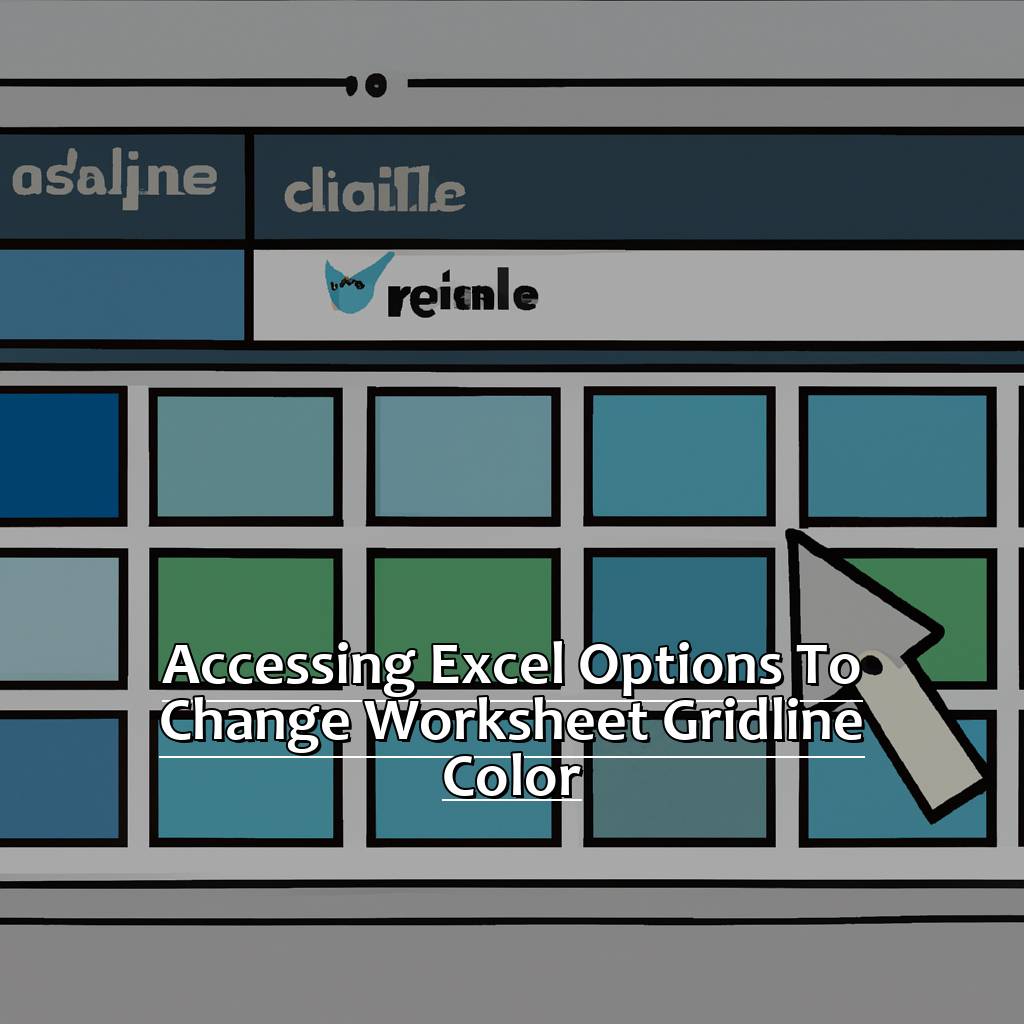
Image credits: manycoders.com by Yuval Washington

Launch Excel

Launch Excel! You can open it from the Start Menu or use a desktop shortcut. When you launch it, you’ll be taken to the start screen. There, you can create a new workbook or open an existing one. To create a new one, click on “Blank Workbook”. To open an existing one, click “Open Other Workbooks” and browse for the file.

When you have your workbook open, you’ll have a blank worksheet. Add your data and customize it to your needs. Depending on your version, some features may be in different places. But, usually, you can access options from the main menu bar at the top.

Changing gridline colors or any other formatting can seem overwhelming. So, practice keyboard shortcuts for easier navigation and time-saving advantages! Instead of launching it from the Start Menu/Desktop shortcut, press <Win key> + R (Run) > type ‘excel’ > press Enter key. This saves a few seconds.

To access advanced settings and design options, go to the ‘File tab’.

Navigate to the File tab

Locate the File tab on the top left corner of your Excel screen, beside the Home tab. Look for a small folder icon. Click on it and you’ll find several options. Look for ‘Options’ and click on it to access Excel Options.

To change gridline colors, select the ‘Advanced’ option from the list on the left-hand side. You’ll see ‘Display options for this worksheet’. Scroll down until you see ‘Gridline color’. Select any of the available colors or create a custom color using RGB codes.

My colleague once used gray gridlines as the default option. But she started seeing errors in her calculations. She realized she had mistakenly reset her default settings back to black gridlines. After she switched back to gray, everything went back to normal!

Let’s talk about selecting options in our next paragraph.

Select Options

To start, click File in the top left corner. This will take you to the backstage view of Excel.

Next, click Options in the left pane.

A page with many options under various categories will appear.

Select the option that suits you or open dialog boxes for further editing.

After making changes/enabling features, click ‘OK’.

Options give access to tools such as a Gallery, Quick Access Toolbar, and Ribbon customization. This includes Add-ins and Macros which help with work-related features and functions.

Excel is a must-have skill to stand out in today’s workforce. However, Gartner reports that AI-powered language processing and analytics software may soon replace jobs done by financial analysts using Excel.

Still, knowledge about Operations in Excel can help with data analysis and visualization for businesses or personal use.

If you want to adjust gridline color in your worksheet, this step-by-step guide can help you change the colors.

Adjusting Gridline Color for Your Worksheet

Excel spreadsheets with unclear or messy gridlines are the worst! Have you experienced difficulty distinguishing columns from rows, or not being able to read the data? Well, you’re in luck! With a few clicks, Excel allows you to customize the gridlines for a more visually appealing worksheet.

In this section, we’ll show you how to adjust the color of your gridlines. We’ll explore the “Advanced” section and look at the display options to help you select the perfect shade.

Image credits: manycoders.com by Adam Washington

Go to Advanced in the left pane

Need to change the color of gridlines in Excel? Here’s a 5-step guide:

1. Click File at the top-left corner.
2. Select Options from the drop-down menu.
3. In the Excel Options dialog box, click Advanced in the left pane.
4. Scroll down to Display options for this worksheet section.
5. Select an option under Gridline color.

Advanced in the left pane offers various options to customize your workbook settings. Under Display options for this worksheet section, you can select settings to make your spreadsheet easier to read and navigate.

Changing the gridline color is a simple way to improve readability and reduce eye strain. Though it may seem minor, it can have a big impact on your workflow efficiency!

Don’t miss out on this optimization. Adjusting gridline colors in Excel is easy and can make your workflow smoother. More customization options are available for further streamlining.

Scroll down to Display options for this worksheet section

Adjusting the gridline color for your Excel worksheet is easy. Find the “Display options for this worksheet section” in the “Page Layout” tab in the ribbon at the top of your workbook. To do this:

1. Click on the “Page Layout” tab in the ribbon.
2. Click on “Gridlines”.
3. Select “More Gridline Colors” from the dropdown list.
4. Scroll down to “Display options for this worksheet section.”

Have a specific shade in mind? Input the RGB value. Choose the color you want and click “OK”. Your changes will be applied immediately.

Gridline colors are a great way to make spreadsheets easier to read and more visually appealing. Team leads can use this feature to quickly differentiate between different sections of data. Try it out today and transform your workbooks!

Choose your preferred color

Ready to change the gridline color of your worksheet? Here’s how!

1. Open your worksheet.
2. Go to the “Page Layout” tab.
3. Select the “Gridlines” dropdown menu in the “Sheet Options” group.
4. Choose “More Gridline Colors” from the dropdown menu.
5. Pick a color from the Standard or Custom tabs in the “Color” dialog box.

You can change the gridline color to any color you like! Red, blue, green, and more! Just remember that printing options may override your changes based on user preferences.

Pro Tip: If the text is difficult to read against dark-colored cells, try using a light-colored gridline.

Ready to apply your chosen gridline color? Click “OK” and you should see the change take effect. You’re done!

Applying Gridline Color Change to Your Worksheet

As an Excel-lover, I understand how important it is to keep worksheets tidy & legible. To make your sheets visually appealing, you can change the color of the gridlines. I’ll show you how!

1. Start by selecting the worksheet tab you want to alter.
2. Then, move to the Page Layout tab & click Sheet Options.
3. Finally, select Gridlines & customize the color of your choice.

In no time, you’ll be able to easily adjust the color of gridlines in your Excel worksheets!

Image credits: manycoders.com by Joel Washington

Choose the worksheet tab you want to modify

When customizing your Excel spreadsheet, selecting the right worksheet tab is essential. You may have multiple worksheets within one workbook, each with different data or purposes. So take a moment to determine which worksheet needs to be adjusted.

Note that depending on your version of Excel, certain steps may vary. But in general, selecting the worksheet should be a simple process.

My coworker once forgot to choose individual sheets before making changes – causing confusion and frustration.

Now, let’s look at how to change the color of the gridlines. Go to the “Page Layout” tab in your Excel window. Then, click on “Page Setup” in the lower right-hand corner of the ribbon. In the “Page Setup” window, select the “Sheet” tab. Under “Gridline color,” choose a new color and click “OK”.

Click the Page Layout tab

Changing the color of worksheet gridlines in Excel? Start by clicking the Page Layout tab. It’s between the Formulas and Review tabs on the ribbon.

Do this in three steps:

1. Open Microsoft Excel and go to the workbook.
2. Find the ribbon at the top of the screen. See the Home, Insert and Data tabs? Click Page Layout.
3. Look for Sheet Options in the Page Layout tab. Check Gridlines.

The Page Layout tab also has other settings, like Margins and Page Setup. Add a background color or watermark? Choose from predefined themes. Or, create custom colors with RGB values.

My classmates and I had trouble changing gridline color. We tried different things until we clicked on “Page Layout.” It gave us access to the grid line properties.

Now that you know how to click on the Page Layout tab, let’s move on. Click the Sheet Options button to change gridline color further.

Click the Sheet Options button

To change the color of your worksheet gridlines in Excel, click the Sheet Options button. This button is located at the bottom-right corner of the “Page Setup” group in the “Page Layout” tab.

To use it, go to the “Page Layout” tab. Find the “Page Setup” group which is usually on the right side of the tab. The Sheet Options button is at the bottom-right corner.

Click the button and a dropdown menu appears. Choose ‘Gridline color’ from the dropdown. Select the color you want.

Clicking the button gives you access to customizing your worksheet’s appearance such as Gridline color and Print Area.

You can create more appealing worksheets with better design elements by changing the gridline color and differentiate from other worksheets that might look similar.

The next step after clicking on Sheet Options button is selecting Gridlines. This will be discussed in the next segment.

Selecting Gridlines allows you to customize their appearance further or just stick with simple changes. This gives you more personalization possibilities when it comes to modifying visuals inside Excel Worksheets.

Select Gridlines

To select gridlines in Excel, follow these steps:

1. Open the worksheet.
2. Click on the ‘Page Layout’ tab. A ribbon with many options will appear.
3. Select the ‘Gridlines’ checkbox. This will open a new menu. Here, choose the desired gridlines.
4. Hide or show them as needed.
5. Click OK to apply them.

Having trouble? Check merged cells or formatting changes. Reset all formatting changes.

Experiment with different types and colors of gridlines. Bold or contrasting colors can be more handy than muted shades.

To make the gridline color change for all worksheets at once, right-click in any cell. Go to ‘Format Cells’. Then click on ‘Fill’ and select the desired ‘Background Colour’.

Changing Gridline Color for All Worksheets

I use Excel spreadsheets a lot. I know it’s important to customize their look. To change the color of gridlines in Excel, I just go to the Home tab. Then I click the Format drop-down menu. From there, I select Gridlines and choose the color I want. It’s a great way to make my data more attractive and easier to read. It’s super easy to do.

Select the Home tab

Time to change the color of gridlines for all worksheets in Excel? Select the Home tab. Here’s the drill:

1. Launch Microsoft Excel on your computer.
2. Open a file or create a new workbook.
3. Find the Home tab at the top of your screen.
4. Look in the Cells group and click the Format button.
5. Select Gridline Color from the Format drop-down menu.

This Home tab houses several groups. Clipboard, Font, Alignment, Number and Cells among others. They assist you in formatting data efficiently.

To change gridline color for all worksheets in Excel, select the Cells group. Then, click Format button. This will offer you choices to format cell properties like font size/style/color/underline effect/borders/cell background etc.

Be aware that if you don’t select any specific worksheet before changing gridline color from Home Tab > Format > Gridline Color – it will affect all existing sheets (even back-end sheets).

Make use of this awesome feature that makes working with multiple worksheets much easier! Follow the steps above to alter gridline colors across spreadsheets quickly & easily.

On to our next topic – Click the Format drop-down menu – where we’ll show you how to find extra formatting options for your worksheets!

Click the Format drop-down menu

Click any cell on your worksheet.

Under the “Home” tab in the ribbon, you’ll find the “Cells” group.

Click the “Format” button below “Cells.”

A drop-down menu will appear – click “Format Cells” to open a new window.

Once open, select the “Border” tab.

At the left-hand side of the pane, select a new color from the selection provided below ‘Color.’

Preview how it looks using the ‘Sample’ section.

You’re not just limited to one worksheet when changing gridline colors in Excel.

You can apply changes to all worksheets with the appropriate settings.

By clicking the Format drop-down menu in any selected worksheet from a workbook of EXCEL 2013 or later version, you can easily format your worksheets without having to manually edit each sheet.

Now you’re ready to choose Gridlines!

Choose Gridlines

To access gridline options, select a cell in one of your worksheets. Navigate to Format > Gridlines > More Gridline Colors. There you can find various colors for your gridlines, standard or custom. To make a custom color, click ‘More Colors’ in the More Gridline Colors window. This will bring up the Custom Colors window. Use the slider controls to create any color you want with Red, Green and Blue (RGB) values.

Borders are ideal for group cells together or frame important info. Select the desired cells then click Home > Font > Border > All Borders.

Font and size also matter. Larger fonts for headers, titles make them stand out. Smaller fonts for body text.

Select your preferred color

Open Excel and head to the “Page Layout” tab. Click “Colors” at the top ribbon menu. Select “Customize Colors” from the drop-down menu. Then, from the “Workbook” section, choose “Gridline Color”. Pick your favorite color from the range of options or click “More Colors” for more choices.

Changing gridline colors is an easy way to customize your Excel spreadsheets. After selecting your preferred shade, all worksheets in that workbook will have identical gridlines.

This can help make data more visible and organized in complex spreadsheets, making it easier to read. In the past, this was viewed as just an aesthetic preference, however, modern design practices now recognize the importance of this feature for reducing eye strain and improving comprehension.

Now, with Excel’s customizations, everyone can get better data visualization that meets their tastes without compromising quality or efficiency.

FAQs about How To Change The Color Of Worksheet Gridlines In Excel